Tuesday, November 29, 2011

R Confidence Intervals and Regions in a linear model

  • for a linear model: \( mm = \beta_0 + \beta_1 x_1 + \beta_2 x_2 + ... + \beta_n x_n \) you can get the confidence intervals of the parameters \( \beta_0 ... \beta_n \)
data(trees)                  ## load the data
mm <- with(trees, lm(Volume ~ Girth + Height)) ## linear model
confint(mm)                  ## get the confidence intervals
2.5 %      97.5 %
(Intercept) -75.68226247 -40.2930554
Girth         4.16683899   5.2494820
Height        0.07264863   0.6058538
[1] "org_babel_R_eoe"
  • the package ellipse provides a command to construct a 2-dimensional confidence region, here we will compute the ellipse for Girth and Height
library(ellipse)
plot(ellipse(mm,c(2,3)),type="l",xlim=c(0,5.5))
points(0,0)
points(coef(mm)[ 2],coef(mm)[ 3],pch=18)
abline(v=confint(mm)[2,],lty=2)
abline(h=confint(mm)[3,],lty=2)


  • we see: (0,0) lies outside the ellipse so we can reject \( H_0 \)
  • the two abline commands produce the lines indicating the one-way confidence intervals, if they were tangential to the ellipse, the CIs would be jointly correct

Monday, November 21, 2011

EBImage

installing

  • EBImage is a part of BioConductor and it is not available on CRAN, so you have to download and install it from the Bioconductor website
  • please type the following as super user (i.e. with admin rights), you will be asked whether you want to update a bunch of packages, answer a - this could take a few minutes
source("http://www.bioconductor.org/biocLite.R")
biocLite("EBImage")

Information about packages

show installed packages

  • show just the names of the installed packages (ordered)
sort(row.names(installed.packages()))
[1] "abind"           "acepack"         "AER"             "akima"          
  [5] "anchors"         "ape"             "base"            "bdsmatrix"      
  [9] "biglm"           "Biobase"         "BiocInstaller"   "bitops"         
 [13] "boot"            "car"             "CarbonEL"        "caTools"        
 [17] "chron"           "class"           "cluster"         "coda"           
 [21] "coda"            "codetools"       "coin"            "colorspace"     
 [25] "compiler"        "CompQuadForm"    "cubature"        "DAAG"           
 [29] "datasets"        "DBI"             "Deducer"         "DeducerExtras"  
 [33] "degreenet"       "Design"          "digest"          "diptest"        
 [37] "doMC"            "doSNOW"          "dynlm"           "e1071"          
 [41] "Ecdat"           "effects"         "ellipse"         "ergm"           
 [45] "fBasics"         "fCalendar"       "fEcofin"         "flexmix"        
...
  • the command installed.packages() provides much more information:
colnames(installed.packages())
[1] "Package"   "LibPath"   "Version"   "Priority"  "Depends"   "Imports"  
 [7] "LinkingTo" "Suggests"  "Enhances"  "OS_type"   "License"   "Built"
  • so if you want to know the package and its version
installed.packages()[,c("Package","Version")] # you can also use the col numbers c(1,3)
Package           Version      
Biobase         "Biobase"         "2.14.0"     
BiocInstaller   "BiocInstaller"   "1.2.1"      
GenABEL         "GenABEL"         "1.6-9"      
multtest        "multtest"        "2.10.0"     
abind           "abind"           "1.3-0"      
acepack         "acepack"         "1.3-3.0"    
AER             "AER"             "1.1-7"      
akima           "akima"           "0.5-4"      
anchors         "anchors"         "3.0-7"      
ape             "ape"             "2.7-1"      
bdsmatrix       "bdsmatrix"       "1.0"        
...
  • show information about a package
packageDescription("multtest")
Package: multtest
Title: Resampling-based multiple hypothesis testing
Version: 2.10.0
Author: Katherine S. Pollard, Houston N. Gilbert, Yongchao Ge, Sandra
        Taylor, Sandrine Dudoit
Description: Non-parametric bootstrap and permutation resampling-based
        multiple testing procedures (including empirical Bayes methods)
        for controlling the family-wise error rate (FWER), generalized
        family-wise error rate (gFWER), tail probability of the
        proportion of false positives (TPPFP), and false discovery rate
        (FDR).  Several choices of bootstrap-based null distribution
        are implemented (centered, centered and scaled,
        quantile-transformed). Single-step and step-wise methods are
        available. Tests based on a variety of t- and F-statistics
        (including t-statistics based on regression parameters from
        linear and survival models as well as those based on
        correlation parameters) are included.  When probing hypotheses
        with t-statistics, users may also select a potentially faster
        null distribution which is multivariate normal with mean zero
        and variance covariance matrix derived from the vector
        influence function.  Results are reported in terms of adjusted
        p-values, confidence regions and test statistic cutoffs. The
        procedures are directly applicable to identifying
        differentially expressed genes in DNA microarray experiments.
Maintainer: Katherine S. Pollard <kpollard@gladstone.ucsf.edu>
Depends: R (>= 2.9.0), methods, Biobase
Imports: survival, MASS
Suggests: snow
License: LGPL
biocViews: Microarray, DifferentialExpression, MultipleComparisons
LazyLoad: yes
Packaged: 2011-11-01 04:28:05 UTC; biocbuild
Built: R 2.14.0; i686-pc-linux-gnu; 2011-11-11 10:32:24 UTC; unix

-- File: /home/mandy/R/i686-pc-linux-gnu-library/2.14/multtest/Meta/package.rds


Thursday, September 15, 2011

R - Rattle rattle gtkin asCairoDevice(da)

Error:
Error in asCairoDevice(da) : Grafik-API Version passt nicht 
or:  
Error in asCairoDevice(da) : Graphics API version mismatch


may be the installation of the package cairoDevice failed.
Try to install the libgtk2.0-dev via sudo apt-get install libgtk2.0-dev


R - install rattle (ubuntu/debian)

First add the line:
        deb http://debian.cran.r-project.org/cran2deb/debian-i386 testing/
or this (for 64 bit vers.)
         deb http://debian.cran.r-project.org/cran2deb/debian-amd64 testing/
to /etc/apt/sources.list

than type: sudo apt-get update

than you can finally install the package via:
sudo apt-get install r-cran-rattle

Saturday, August 20, 2011

R - R2OpenBUGS

download linux source
R CMD INSTALL BRugs_0.7.1.tar.gz
download windows binaries than install it as a local package (in the menu)


more information here

R - par() change the position of axes labels and tick marks

  • create a example plot using the trees data set
head(trees)
  Girth Height Volume
1   8.3     70   10.3
2   8.6     65   10.3
3   8.8     63   10.2
4  10.5     72   16.4
5  10.7     81   18.8
6  10.8     83   19.7
  • now we create the plot (girth on the x-axis, heigth on the y-axis, size and color of the circles indicating the volume of the trees):
my.col <- rainbow(100, start=0.3,end=0.9) ## provid an vector with colors
with(trees, symbols(Girth,Height, circles=Volume/30, bg=my.col[Volume], inches=0.3)) ## plot the example plot (symbols plot) 

  • now we save the current par()-settings (for recovering) - and so we can restore it later
my.old.par <- par()
  • the mgp controls the position of the axes labels, and tick labels and the axes
  • default value c(3,1,0)
  • the first entry controls the position of the axis labels, the second the position of the tick labels
par(mgp=c(-2,-1,0))
with(trees, symbols(Height, Girth, circles=Volume/30, bg=my.col[Volume], inches=0.3, main="Trees") )

  • so if we change the first two values of mgp to negative numbers the axis labels and the tick labels are now located in the inner region
  • the absolute value define the distances, so we try this second example:
par(mgp=c(-2,-3,0))
with(trees, symbols(Height, Girth, circles=Volume/30, bg=my.col[Volume], inches=0.3, main="Trees") )

  • the third element of mgp controls the axes and it have the same effect, every value different from zero moves the axes
par(mgp=c(-2,-3,-1))
with(trees, symbols(Height, Girth, circles=Volume/30, bg=my.col[Volume], inches=0.3, main="Trees") )

my.col <- rainbow(100, start=0.3,end=0.9) ## provid an vector with colors
with(trees, symbols(Height, Girth, circles=Volume/30, bg=my.col[Volume], inches=0.3)) ## plot the example plot (symbols plot) 
  • if you want to change just the orientation of the ticks use tcl
  • tcl defines the length of tick marks as a fraction of the height of a line of text
  • default ist -0.5
  • if you use a positive value the orientation is changed
par(mgp=c(3,1,0),tcl=0.5) ### set mgp back to default, change tcl
with(trees, symbols(Height, Girth, circles=Volume/30, bg=my.col[Volume], inches=0.3, main="Trees") )

Saturday, August 13, 2011

R - extract year, month etc.... from date

extract year, month, day… from date

  • create vector of dates in standard format
my.dates <- as.Date(format(ISOdatetime(2000:2009,1:10,1:5,0,0,0),"%Y-%m-%d"))
my.dates
 [1] "2000-01-01" "2001-02-02" "2002-03-03" "2003-04-04" "2004-05-05"
 [6] "2005-06-01" "2006-07-02" "2007-08-03" "2008-09-04" "2009-10-05"
(make sure your object is of date fromat, check it with str(your.object)
  • extract years using format:
my.years <- format(my.dates,"%Y") # %y without century
my.years
 [1] "2000" "2001" "2002" "2003" "2004" "2005" "2006" "2007" "2008" "2009"
  • or months
my.months <- format(my.dates,"%m")
my.months
 [1] "01" "02" "03" "04" "05" "06" "07" "08" "09" "10"
  • or names of month (in current local)
my.months <- format(my.dates,"%b") # %B for long form
my.months
 [1] "Jan" "Feb" "Mär" "Apr" "Mai" "Jun" "Jul" "Aug" "Sep" "Okt"
  • or days (of month)
my.days <- format(my.dates,"%d")
my.days
 [1] "01" "02" "03" "04" "05" "01" "02" "03" "04" "05"
  • or week day (in current local)
my.days <- format(my.dates,"%a") # %A for long form, %w (0-6) of %u (1-7) for number
my.days
 [1] "Sa" "Fr" "So" "Fr" "Mi" "Mi" "So" "Fr" "Do" "Mo"
  • or day of year
my.days <- format(my.dates,"%j")
my.days
 [1] "001" "033" "062" "094" "126" "152" "183" "215" "248" "278"
  • or week of year (sunday as first day of the week)
my.weeks <- format(my.dates,"%U") # %W for monday = first day of the week
my.weeks
 [1] "00" "04" "09" "13" "18" "22" "27" "30" "35" "40"
  • local format of date
my.days <- format(my.dates,"%x")
my.days
 [1] "01.01.2000" "02.02.2001" "03.03.2002" "04.04.2003" "05.05.2004"
 [6] "01.06.2005" "02.07.2006" "03.08.2007" "04.09.2008" "05.10.2009"

R - subscripting 3

subsetting with logical indices

  • elements corresponding to a TRUE in the subscript vector are selected, those corresponding to a FALSE are excluded, NAs in the the logical subscript vector produce NAs
my.vector <- letters[1:10] # vector of a...j
my.vector
 [1] "a" "b" "c" "d" "e" "f" "g" "h" "i" "j"
my.index <- rep(c(TRUE,FALSE),5) # the subscript vector (of length 10)
my.index
 [1]  TRUE FALSE  TRUE FALSE  TRUE FALSE  TRUE FALSE  TRUE FALSE
my.vector[my.index]
[1] "a" "c" "e" "g" "i"
  • if the subscript vector consists of less elements than the subscripted vector, it is repeated as many times as necessary (warning if the the vector length is not a multiple of the length of the subscript vector)
short.index <- c(T,F) # T is the same as TRUE, F as FALSE
short.index
[1]  TRUE FALSE
my.vector[short.index] # has the same result as above
[1] "a" "c" "e" "g" "i"
  • if the subscript vector is longer than the vector for every TRUE or NA entry without target a NA is produced
short.vector <- letters[1:3]
short.vector
[1] "a" "b" "c"
my.index <- rep(c(T,F,NA),2)
my.index
[1]  TRUE FALSE    NA  TRUE FALSE    NA
short.vector[my.index]
[1] "a" NA  NA  NA

R - subscripting 2

subsetting with character indices - vectors and lists

  • extract elements of named vectors, lists
named.x <- 1:10  # produce a vector containing the numbers 1...10
named.x   #  has no names yet
 [1]  1  2  3  4  5  6  7  8  9 10
  • if the object has no names, NAs are produced
named.x["one"]
[1] NA
  • name the vector:
names(named.x) <- c("one","two","three","four","five","six","seven","eight","nine","ten")
named.x
  one   two three  four  five   six seven eight  nine   ten 
    1     2     3     4     5     6     7     8     9    10
  • now it works
named.x["one"]
one 
  1
  • if names are duplicated only the first match is returned (the value with the lowest index)
names(named.x)<-rep(c("one","two","three","four","five"),rep(2,5))
named.x
  one   one   two   two three three  four  four  five  five 
    1     2     3     4     5     6     7     8     9    10
named.x[c("one","two","three")]
  one   two three 
    1     3     5
  • NA is returned if a name do not match any element
named.x["twenty"]
<NA> 
  NA
  • NA is returned if a subscript is character NA
named.x[c("one",NA,"three")]
  one  <NA> three 
    1    NA     5
  • to find all occurences one can use %in% and then subset with the logical vector (you can do this in one step)
named.x[names(named.x) %in% c("one","two")]
one one two two 
  1   2   3   4

Tuesday, August 2, 2011

Monday, August 1, 2011

R - subscripting

subsetting

  • creating a list for examples
myl <- list(one=10,two=20,three=30)
myi <- "one"
one
  • subsetting is carried out with three different operators:
    • dollar: $
    • square bracket: [
    • double square bracket: [[
  • these are generic functions
  • there are four basic types of subscript indices
    • positive integers
    • negative integers
    • logical vectors
    • character vectors
  • the first (left-most) index moves the fastest, the right-most index is the slowest (so a matrix is filled column by column)

the square bracket

  • the returned value is of the same type of the value it is applied to
myl[c(1,2)]
10 20
  • evaluate its second argument
myl[myi]
10
  • does not use partial matching when extracting named elements
myl["on"]
  • cannot be used for subscripting environments

the double square bracket

  • extract a single value
myl[[1]]
10
  • evaluate its second argument
myl[[myi]]
10
  • does not use partial matching when extracting named elements
myl[["on"]]

the dollar

  • extract a single value
myl$two
20
  • does not evaluate its second argument
myl$myi
  • uses partial matching extracting named elements
myl$on
10
  • cannot be used for subscripting atomic vectors

subsetting with positive indices

  • vector of positive integer values to indicate the set to be extracted
myv <- 1:10 
myi <- c(2,4,7)
myv[myi]
myv[c(2,4,7)]
[1] 2 4 7
[1] 2 4 7
  • if the subscript is larger than the length of the vector, NAs are produce
myv[c(1,11,3)]
[1]  1 NA  3
  • NA as subscript produces also a NA
myv[c(1,11,NA)]
[1]  1 NA NA
  • zero as subscript will be ignored
myv[c(1,2,0,3)]
[1] 1 2 3
  • if the subscript vector has the length zero, the result is also of length zero
myi <- numeric()
myv[myi]
integer(0)
  • example: select elements which have even numbered subscripts
v <- rnorm(20)
myi <- seq(2,length(v),by=2)
myi
v[myi]
 [1]  2  4  6  8 10 12 14 16 18 20
 [1]  0.35380115 -0.02156840 -1.51804278  0.38278037  0.03867578 -1.25803279
 [7]  0.62863255  0.07111270 -0.73416837  0.18966622

subsetting with negative indices

  • subscript vector consists of negative integer values indicating the indices not to be extracted
  • zero as subscript will be ignored
myv[-c(1,2,0,3)]
[1]  4  5  6  7  8  9 10
  • NAs are not allowed
myv[-c(1,NA,3)]
Error in myv[-c(1, NA, 3)] : 
  nur Nullen dürfen mit negativen Indizes gemischt werden
  • zero length subscript produces zero length result
myv <- 1:10 
myi <- numeric()
myv[-myi]
 integer(0)
  • positive and negatives subscripts cannot be mixed

to be continued... (most parts taken from Gentleman, R Programming for Bioinformatics) …

Tuesday, July 26, 2011

R - recode() data

recode() - from package lordif

library(lordif)  # maybe you have first to install the package (install.packages("lordif"))
  • creating example data
z <- sample(0:1, 25, replace=T)
original <- c(0,1)
new <- c("boy", "girl")
z
original
new
z:  1 1 1 0 0 0 1 1 1 1 0 0 1 1 1 1 0 1 1 1 1 1 1 1 0
original: 0 1
new:  "boy"  "girl"
  • so z is a vector consisting of 1 and 0
  • original contains the distinct values of z
  • and new contains the values which should replace the original values in the following way: the first item of original is replaced by the first value of new, the second by the second etc pp
z <- recode(z, original, new)
z
 [1] "girl" "girl" "girl" "boy"  "boy"  "boy"  "girl" "girl" "girl" "girl"
[11] "boy"  "boy"  "girl" "girl" "girl" "girl" "boy"  "girl" "girl" "girl"
[21] "girl" "girl" "girl" "girl" "boy"

u

Wednesday, July 20, 2011

R - t.test for subsets of a data frame (ddply or tapply)

(two sample t-test for groups in data frame here)
First we create a data frame, on which we can work
x <- rnorm(100)                 
y <- sample(1:3, 100, replace=T)
z <- sample(1:2, 100, replace=T)

df <- data.frame(group=y,sex=z,sds=x)
head(df)
group sex       sds
1     1   2 1.3412663
2     1   1 0.8000326
3     2   2 0.0371029
4     1   2 0.2064684
5     1   2 1.6429816
6     3   1 1.3271138
In the following I use ddply() from the plyr-package, so if you did not install and/or load it you have to do it now - the command library() without any argument gives you a list of the installed packages:
install.packages("plyr") # install the package
library(plyr) # load it
Here is the function for doing the t.tests:
t.test.plyr <- function(x, var, mean=0 ){
  y <- rep(NA,10)
  y[6] <- nrow(x)[1]              # count observations
  if(nrow(x) < 2) return(y)       # exits if too less observations
  res <- t.test(x[var], mu=mean)  # doing the test

  y[1] <- res$statistic           # extract values of interest
  y[2] <- res$p.value      
  y[3] <- res$estimate     
  y[4] <- res$conf.int[1]  
  y[5] <- res$conf.int[2]  
  y[7] <- res$parameter    
  y[8] <- res$method       
  y[9] <- res$alternative  
  y[10] <- res$null.value   

  names(y) <- c("statistic","p.value","estimate","conf.int1", "conf.int2", "nobs","dof","method","alternative","null.value")
  y 
}

where t.test.plyr() is a function of:
- x - the data frame
- var - the variable which should be testet
- mean - the mean of the t-test

now we can use ddply in the following way:
result <- ddply(df, .(group, sex), t.test.plyr, "sds")
result
group sex           statistic           p.value            estimate
1     1   1   0.774917157596946 0.445379429071851   0.132214420988956
2     1   2  -0.415594591752269  0.68359099812399 -0.0987341821354776
3     2   1   0.130257003222609 0.899578855830346  0.0602600950757679
4     2   2 -0.0579045286518569 0.954965406753824 -0.0150105343694587
5     3   1    1.18044920537142 0.256202807853187   0.406567809727671
6     3   2    1.49215606704641  0.15126489039304   0.294865619363907
           conf.int1         conf.int2 nobs dof            method alternative
1 -0.218494854049804 0.482923696027717   27  26 One Sample t-test   two.sided
2 -0.605109702463049 0.407641338192093   16  15 One Sample t-test   two.sided
3  -1.00655416438508  1.12707435453662    9   8 One Sample t-test   two.sided
4 -0.592608791299465 0.562587722560548   11  10 One Sample t-test   two.sided
5 -0.327541518602652  1.14067713805799   16  15 One Sample t-test   two.sided
6 -0.117342538637965  0.70707377736578   21  20 One Sample t-test   two.sided
  null.value
1          0
2          0
3          0
4          0
5          0
6          0
If you want to change the mu in you t.test, add the argument mean:
result <- ddply(df, .(group, sex), t.test.plyr, "sds", mean=1)
result
If there is no need or you do not want a data frame as result you can just use tapply(). tapply results in a list with as many elements as subsets, each element contains the results of each t.test (as list).
res <- tapply(df$sds, list(df$sex,df$group), t.test)
res
1      2      3     
1 List,9 List,9 List,9
2 List,9 List,9 List,9
So the first element of res contains the t.test results for sex=1 and group=1 etc pp
res[[1]]
One Sample t-test

data:  X[[1L]] 
t = 0.7749, df = 26, p-value = 0.4454
alternative hypothesis: true mean is not equal to 0 
95 percent confidence interval:
 -0.2184949  0.4829237 
sample estimates:
mean of x 
0.1322144

Friday, July 15, 2011

Ubuntu - convert pdf to images (resolution selectable)

nice command line tool:
pdftoppm

creates one image (png, jpeg pbm or pgm) per page.

e.g. if source.pdf has two pages
pdftoppm -png -r 600 source.pdf target
creates 2 images, solution: 600 DPI, file names: target-01.png, target-02.png

Thursday, July 14, 2011

Emacs - change style of word wrapping

use word wrap
M-x visual-line-mode
Emacs displays long lines by truncation
M-x toggle-truncate-lines

VBA excel - sheets exist ?

The function:
Public Function SheetExists(SheetName As String) As Boolean
    Dim ws As Worksheet
    SheetExists = False
    For Each ws In ThisWorkbook.Worksheets
        If ws.Name = SheetName Then SheetExists = True
    Next ws
End Function
create sheet if it does not exist:
For i = 1 to n
    If SheetExists("Sheet" & CStr(i)) Then
        MsgBox ("Sheet" & CStr(i) & " exists")
    Else
        Worksheets.Add(After:=Worksheets(Worksheets.Count)).Name = "Sheet" & CStr(i)
    End If
Next i

Saturday, July 9, 2011

R ggplot - barplot

barplot

  • load the package ggplot2 and the diamond data
  • first we create a object p of class ggplot, where we map clarity to x (horizontal position)
p <- ggplot(diamonds, aes(x=clarity))
summary(p)
data: carat, cut, color, clarity, depth, table, price, x, y, z
  [53940x10]
mapping:  x = clarity
faceting: facet_grid(. ~ ., FALSE)
  • p contains all information ggplot needs to build a barplot, all we have to do is adding a layer with geom="bar";
p + layer(geom="bar")

  • to this simple barplot we can add the following (optional) aesthetics:
    • colour: color of the borders of the bins
    • fill: color of the filling
    • size:
    • linetype: line type of the borders
    • weight:
    • alpha: transparency of fill [0,1]
p + layer(geom="bar", geom_params=list(fill="steelblue", colour="black", linetype=4, alpha=0.3))

  • but a barplot can visualize more information about the data - so we add a new mapping to p
p <- ggplot(diamonds, aes(x=clarity, fill=color)) # where color is the variable of the dataframe diamonds
  • now the default output looks like:
p + layer(geom="bar")

  • the plot can be customized by the same aesthetics, fill would override the aesthetic mapping of p
  • additional we can add a position adjustment
p + layer(geom="bar", position="dodge") 

  • or
p + layer(geom="bar", position="fill") 

  • if we flip (coordflip()) the underlying coordinate system, we can rotate the plot
p + layer(geom="bar", position="stack") + coord_flip()

  • or we even can change the coordinate system to polar coordinates:
p + layer(geom="bar", position="stack") + coord_polar()

R - filled.contour plot

filled.contour

  • if you have a matrix with nxm dimensions and every entry represents a value of interest and the indices of the entry describe the position, then you can use filled.contour() to visualize the matrix
  • first we create a simple matrix to demonstrate how it works:
x <- y <- 1:10 # create two vectors with the integers from 1 to 10
z <- outer(x,y) # create a matrix as the outer product of the two vectors
z # show the matrix
      [,1] [,2] [,3] [,4] [,5] [,6] [,7] [,8] [,9] [,10]
 [1,]    1    2    3    4    5    6    7    8    9    10
 [2,]    2    4    6    8   10   12   14   16   18    20
 [3,]    3    6    9   12   15   18   21   24   27    30
 [4,]    4    8   12   16   20   24   28   32   36    40
 [5,]    5   10   15   20   25   30   35   40   45    50
 [6,]    6   12   18   24   30   36   42   48   54    60
 [7,]    7   14   21   28   35   42   49   56   63    70
 [8,]    8   16   24   32   40   48   56   64   72    80
 [9,]    9   18   27   36   45   54   63   72   81    90
[10,]   10   20   30   40   50   60   70   80   90   100
  • now let us plot the matrix:
filled.contour(z)

  • the matrix is mapped to a 1x1 square: the entry with the indices (1,1) and the value 1 to the point with the coordinates (0,0) and the entry with the indices (10,10) and the value (100) to the points with the coordinates (1,1); if you want to change the axes you can add a x and a y argument to the plot;so let's use the vectors x and y from above (with the entries 1 to 10) and also change to colors
  • filled.contour() uses the cm palette as default (cyan for low, magenta for heigh values);
filled.contour(x=x,y=y,z, col=heat.colors(20))

  • more palettes you find here

And a last example

my.seq <- seq(-pi, pi, length=50) # creating a vector as a sequence from 0 to 2*pi with 50 entries
my.seq2 <- seq(-0.5*pi, 1.5*pi, length=50) # creating a vector as a sequence from 0 to 2*pi with 50 entries
my.matrix <- outer(sin(my.seq),cos(my.seq2)) # creating the matrix using sin, cos and outer
filled.contour(x=my.seq, y=my.seq2,my.matrix, plot.title=title(main="Products Sin(x)*Cos(y) on [-Pi,Pi]x[-0.5Pi,1.5Pi]", xlab="x", ylab="y"), key.title=title(main="products"), col=terrain.colors(20))

Latex Beamer - package beamercolor

Manual.
You can download the .sty file: here BeamerColor.sty
create a folder in your latex file directory
/usr/share/texmf-texlive/tex/latex/
the path can differ from the path above (e.g. if you use TeTeX).
copy the example.sty file in this directory
cp /home/me/pathtopackage/example.sty /usr/share/texmf-texlive/tex/latex/

run
sudo mktexlsr
add the line \usepackage{example} to you document

Friday, July 8, 2011

RExcel - do not work after installing new R version

When a new version of R is installed, a few things have to be done.

rcom and rscprooxy have to be installed in the new version.
 install.packages(c("rcom", "rscproxy")) 

the line
library(rcom) 
has to be added to the etc\RProfile.site (standard path Win: C:\Programme\R\R-Version\etc\)

comRegisterRegistry() has to be run (in the new version)

bin\RSetReg.exe has to be run  (path Win: C:\Programme\R\R-2.12.1\bin\i386)

Thursday, July 7, 2011

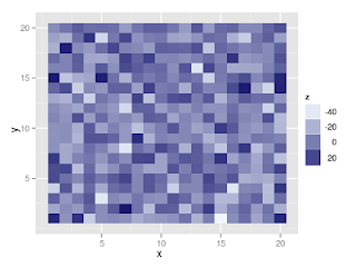
R ggplot2 - simple heatplot

simple heatplot

  • load the library ggplot2, if you have not installed it yet - install it via install.packages("ggplot2")
  • create the example data frame
  • map it to the plot
x <- rep(1:20,20)
y <- rep(1:20, rep(20,20))
z <- rnorm(400, mean=0, sd=15)
df <- data.frame(x=x,y=y,z=z)
ggplot(df, aes(x=x,y=y, fill=z)) + geom_tile()

  • now we can change the colors (colorchart) by add a scale_fill_gradient(low="green", high="red")
ggplot(df, aes(x=x,y=y, fill=z)) + geom_tile()+scale_fill_gradient(low="green", high="red")

  • an a second one (with more soothing colors)
ggplot(df, aes(x=x,y=y, fill=z)) + geom_tile()+scale_fill_gradient(low="aliceblue", high="midnightblue")

Emacs - make buffer names unique - eindeutige Buffernamen

  • add the line 
(require 'uniquify)

to your emacs configuration file ( .emacs in your home directory )

  • restart emacs
  • type: M-x customize-option
  • then choose the variable: uniquify-buffer-name-style
  • set it to one of these: forward or reverse or post-forward or post-forward-angle-brackets (just hit Enter)
  • set for the current session and save for future sessions then exit

R - add a table to a plot

addtable2plot()

  • suppose you have a vector with different dates of events and you want to investigates if there are month with more or less events, the first step maybe is to draw a barplot
  • so let us generate first a vector with the different dates:
  • and than we create a vector with the extracted month (as factor)
my.dat <- as.Date(sample.int(500, 1000, replace=T), origin="2000-01-01") 
# extract month, use the abbreviated form of months
my.months <- months(my.dat, abbreviate=T)
df <- data.frame(date=my.dat, month=my.months)
table(df$month) 
Apr Aug Dez Feb Jan Jul Jun Mai Mär Nov Okt Sep 
122  72  66 103 121  61  51  85 129  59  64  67
  • as one can see the month are in alphabetical order so we have to correct this
  • therefore we use ISOdatetime and format for creating a vector of the 12 months in the correct order and use this vector for creating a labeled factor out of df$month
df$month <- factor(df$month, levels=format(ISOdatetime(2000,1:12,1,0,0,0),"%b"))
# show the first 50 elements of my.
table(df$month)
Jan Feb Mär Apr Mai Jun Jul Aug Sep Okt Nov Dez 
121 103 129 122  85  51  61  72  67  64  59  66
  • now we can create hour barplot (use the package plotrix)
# if it is not installed yet, install it via install.packages("plotrix")
# load the package
library(plotrix) 

# create the table for plotting (the same as above)
my.table <- with(df, table(month)) # equivalent to table(df$month)
# plot it! (choosing the color from here)

barp(my.table, col=colors()[c(462:471,473,477)], xlab="Month", ylab="count")

  • now we create the same plot but add the table
# create the table for the plot - i want the horizontal table so i have to transpose it
m2 <- t(as.matrix(my.table)) 
# barplot
barp(my.table, col=colors()[c(462:471,473,477)], xlab="month", ylab="count")
# add the table: the first two arguments are the position relative to the coord system of the plot
# the third argument is the table (a data frame or a matrix), the bty: "o" draw a box, "n" no box
# bg is the argument for the background 
addtable2plot(3,140,m2, bty="o", bg="aliceblue")

now add the table with ggplot2


require(gridExtra)
require(ggplot2)
# generate random dates
my.dat <- as.Date(sample.int(500, 1000, replace=T), origin="2000-01-01") 
# extract month
my.months <- factor(month(my.dat),levels=1:12,labels=month.abb)
df <- data.frame(date=my.dat, month=my.months)

# prepare table
mytable <- tableGrob(t(as.data.frame(table(df$month))),show.rownames = F,show.colnames = F)

ggplot(df,aes(x=month,fill=month)) +
    geom_bar() +
    ylim(0,150) +
    annotation_custom(mytable,xmin = 4.5,xmax=15,ymin=130,ymax = 150) +
    scale_fill_manual(values=colors()[c(462:471,473,477)],guide="none")
ggsave("tabletoplot.png")


R - generate a vector with names of months (like LETTERS)

> format(ISOdatetime(2000,1:12,1,0,0,0),"%b")
gives:
 [1] "Jan" "Feb" "Mrz" "Apr" "Mai" "Jun" "Jul" "Aug" "Sep" "Okt" "Nov" "Dez"
where the month names depend on local settings. If you use %B instead of %b you get the non abbreviated months. How ever, there is also an easier way if you want the months in English: the vector
> month.name
 
gives
 [1] "January"   "February"  "March"     "April"     "May"       "June"     
 [7] "July"      "August"    "September" "October"   "November"  "December" 
or
> month.abb
 
gives
 [1] "Jan" "Feb" "Mar" "Apr" "May" "Jun" "Jul" "Aug" "Sep" "Oct" "Nov" "Dec"

Wednesday, July 6, 2011

R - ddply

ddply

dataframe in dataframe out

example

  • first we create a data frame with the following columns: id, date, value
  • to create the id column we use rep(), where the first argument 1:5 (the vector (1,2,3,4,5)) is repeated five times, so we have a vector with length 25
  • the vector dates is generated in the following way:
    • generate a vector of random numbers between 1 and 1500 and length 25 (sample.int())
    • use as.Date with the origin argument, this converts the integers into Date, where the the origin is day 0 (in the case 0 is convert to the origin i.e. 2000-01-01, 1 is mapped to 2000-01-02 etc pp, so we get a vector of dates between 2000 and beginning 2005
  • vals are generated by the random numbers function rnorm() (normal distributed with mean 5 and standard deviation 1
  • last but not least put the three together in one data frame (and let us show the first lines)
id <- rep(1:5,5)
dates <- as.Date(sample.int(1500, 25, replace=T), origin="2000-01-01") 
vals <- rnorm(25, mean=5, sd=1)
df <- data.frame(id=id, date=dates, val=vals)
head(df)
  id       date      val
1  1 2001-12-31 5.778680
2  2 2002-08-02 6.982799
3  3 2002-04-23 5.925903
4  4 2000-08-03 3.527375
5  5 2002-08-29 5.239211
6  1 2003-01-28 5.118337
  • id encodes a person, date contains the day of the measurement and val the values
  • now we want to add a column which contains the the first measurement in time
  • therefore we had to load plyr, then we use the function ddply() (the meaning of the first two letters is data frame in data frame out)
  • the first argument of the function is the data frame we pass to ddply
  • the second argument defines the groups (we want the min of each person so our grouping variable is id)
  • transform says we want to change existing data frame - like recode a variable or add a new (another choice would be summarise - if we want to aggregate the data) - so we add a variable named start and it should be the min() of our date per person
res <- ddply(df, .(id), transform, start=min(date))
res
iddatevalstart
12001-12-315.778679592025192001-03-07
12003-01-285.118336553288972001-03-07
12003-11-143.750754634375052001-03-07
12001-03-073.363050937734682001-03-07
12001-03-076.61415837892332001-03-07
22002-08-026.982798845791672000-05-29
22003-12-305.44500191386462000-05-29
22000-05-295.925679827166672000-05-29
22000-11-264.601699565975442000-05-29
22002-08-045.023958124582000-05-29
32002-04-235.925903245936592000-02-02
32003-04-286.592460569591672000-02-02
32002-10-205.897804643006622000-02-02
32000-02-024.05486188162692000-02-02
32000-05-305.47226334023782000-02-02
42000-08-033.527374580480372000-08-03
42002-11-023.988538941622852000-08-03
42002-11-134.543730885196552000-08-03
42003-08-024.21442451843462000-08-03
42003-12-194.987674782982792000-08-03
52002-08-295.239211212098212000-04-27
52000-04-274.204002414119612000-04-27
52003-07-266.18219572726462000-04-27
52003-05-184.535154046383622000-04-27
52001-07-233.066952749405012000-04-27
  • if we change the function just a little we get the days elapsed from the first measurment:
res <- ddply(df, .(id), transform, dayselapsed=date-min(date))
res
iddatevaldayselapsed
12001-12-315.77867959202519299
12003-01-285.11833655328897692
12003-11-143.75075463437505982
12001-03-073.363050937734680
12001-03-076.61415837892330
22002-08-026.98279884579167795
22003-12-305.44500191386461310
22000-05-295.925679827166670
22000-11-264.60169956597544181
22002-08-045.02395812458797
32002-04-235.92590324593659811
32003-04-286.592460569591671181
32002-10-205.89780464300662991
32000-02-024.05486188162690
32000-05-305.4722633402378118
42000-08-033.527374580480370
42002-11-023.98853894162285821
42002-11-134.54373088519655832
42003-08-024.21442451843461094
42003-12-194.987674782982791233
52002-08-295.23921121209821854
52000-04-274.204002414119610
52003-07-266.18219572726461185
52003-05-184.535154046383621116
52001-07-233.06695274940501452

Saturday, June 25, 2011

R - get back the last result (if it was forgotten to assign it)

R stores the result of the LAST operation in .Last.value; So, for example, if you read a file into R and forgot to assign it,
x <- .Last.value 
helps you, without reading it again..., it is the same for the result of every other function

R - working with unique() and duplicated()

duplicated() vs. unique()

  • first we create a vector we can work with:
x <- sample(LETTERS[1:10], 20, replace=T)
x
 [1] "J" "C" "J" "C" "F" "J" "E" "J" "H" "A" "C" "G" "I" "A" "F" "H" "J" "C" "C"
[20] "D"
  • unique() gives us a vector containing every new element of x but ignores repeated elements
unique(x)
[1] "J" "C" "F" "E" "H" "A" "G" "I" "D"
  • duplicated() gives a logical vector
duplicated(x)
 [1] FALSE FALSE  TRUE  TRUE FALSE  TRUE FALSE  TRUE FALSE FALSE  TRUE FALSE
[13] FALSE  TRUE  TRUE  TRUE  TRUE  TRUE  TRUE FALSE
  • so if we want to get the same result like the one from unique we have to index x in the following way:
x[duplicated(x)==F]
[1] "J" "C" "F" "E" "H" "A" "G" "I" "D"
  • if we want to get just repeated occurences (i.e. a vector without the first occurence) we use the following line
x[duplicated(x)==T]
 [1] "J" "C" "J" "J" "C" "A" "F" "H" "J" "C" "C"
  • we can use these commands the same way on dataframes, so let our x code persons, and we add a numeric value which could be a measurement and the order of the vector describes the order in which the measurements are taken
y  <- rnorm(20, mean=10)
df <- data.frame(person=x, meas=y)
df
   person      meas
1       J 11.180452
2       C 10.235697
3       J 10.908622
4       C 10.677399
5       F  8.564007
6       J 10.070557
7       E 10.144191
8       J 10.872314
9       H 11.635032
10      A 10.448090
11      C 10.642052
12      G  8.689660
13      I 10.007930
14      A  8.321125
15      F 10.610739
16      H  9.060412
17      J 10.678726
18      C  8.513766
19      C  8.851564
20      D 12.793154
  • we extract the first measurement of each person with (the comma behind the F is important - it says we want the whole line)
df[duplicated(df$person)==F,]
   person      meas
1       J 11.180452
2       C 10.235697
5       F  8.564007
7       E 10.144191
9       H 11.635032
10      A 10.448090
12      G  8.689660
13      I 10.007930
20      D 12.793154
  • and with the following command we can extract the follow up measurements
df[duplicated(df$person)==T,]
   person      meas
3       J 10.908622
4       C 10.677399
6       J 10.070557
8       J 10.872314
11      C 10.642052
14      A  8.321125
15      F 10.610739
16      H  9.060412
17      J 10.678726
18      C  8.513766
19      C  8.851564
  • we also can use duplicate in a recursive way; the result of the following function is a list containing vectors whereupon the first contains the first occurence, the second the second, etc.; you can change it easily: so it can give back logical vectors which can use to index a dataframe, or for working on a dataframe itself (which both would be more useful)
sep.meas <- function(dupl){
  res <- list()
  while(length(dupl)>0){
    res[[length(res)+1] ] <- dupl[duplicated(dupl)==F]
    dupl <- dupl[duplicated(dupl)==T]
  }
 res
}
  • if we use it on x we get the following result
sep.meas(x)
[[1]]
[1] "J" "C" "F" "E" "H" "A" "G" "I" "D"

[[2]]
[1] "J" "C" "A" "F" "H"

[[3]]
[1] "J" "C"

[[4]]
[1] "J" "C"

[[5]]
[1] "J" "C"

R - sorting vectors: sort() vs. order()

sort() and order()

  • both operates on vectors and has the same aim, but the results are very different
First we create a vector we can sort:
x <- sample(LETTERS[1:10], 100, replace=T) # create a vector to sort by sampling from the first 10 Letters of the alphabet 100 times
x
  [1] "H" "D" "I" "E" "F" "B" "E" "G" "D" "A" "H" "I" "E" "A" "E" "A" "I" "J"
 [19] "I" "A" "B" "F" "A" "I" "F" "B" "A" "H" "J" "A" "E" "A" "C" "A" "A" "C"
 [37] "F" "C" "D" "G" "I" "I" "B" "J" "J" "D" "I" "J" "G" "J" "A" "B" "B" "C"
 [55] "A" "B" "D" "E" "D" "D" "E" "J" "A" "J" "G" "D" "A" "B" "D" "I" "F" "H"
 [73] "D" "J" "D" "E" "E" "A" "A" "J" "B" "E" "C" "I" "C" "F" "F" "E" "E" "J"
 [91] "H" "H" "F" "I" "A" "I" "H" "I" "I" "I"
  • the result of sort() is a vector consisting of elements of the original (unsorted) vector
sort(x)
  [1] "A" "A" "A" "A" "A" "A" "A" "A" "A" "A" "A" "A" "A" "A" "A" "A" "A" "B"
 [19] "B" "B" "B" "B" "B" "B" "B" "B" "C" "C" "C" "C" "C" "C" "D" "D" "D" "D"
 [37] "D" "D" "D" "D" "D" "D" "D" "E" "E" "E" "E" "E" "E" "E" "E" "E" "E" "E"
 [55] "E" "F" "F" "F" "F" "F" "F" "F" "F" "G" "G" "G" "G" "H" "H" "H" "H" "H"
 [73] "H" "H" "I" "I" "I" "I" "I" "I" "I" "I" "I" "I" "I" "I" "I" "I" "I" "J"
 [91] "J" "J" "J" "J" "J" "J" "J" "J" "J" "J"
  • if we do the same with order the result is completely different - we get a vector with the ordered indices of the original (unsorted) vector
order(x)
  [1]  10  14  16  20  23  27  30  32  34  35  51  55  63  67  78  79  95   6
 [19]  21  26  43  52  53  56  68  81  33  36  38  54  83  85   2   9  39  46
 [37]  57  59  60  66  69  73  75   4   7  13  15  31  58  61  76  77  82  88
 [55]  89   5  22  25  37  71  86  87  93   8  40  49  65   1  11  28  72  91
 [73]  92  97   3  12  17  19  24  41  42  47  70  84  94  96  98  99 100  18
 [91]  29  44  45  48  50  62  64  74  80  90
  • if you want to get the ordered vector (like with sort()) you have to index the original vector with the vector of the indices
x[order(x)]
  [1] "A" "A" "A" "A" "A" "A" "A" "A" "A" "A" "A" "A" "A" "A" "A" "A" "A" "B"
 [19] "B" "B" "B" "B" "B" "B" "B" "B" "C" "C" "C" "C" "C" "C" "D" "D" "D" "D"
 [37] "D" "D" "D" "D" "D" "D" "D" "E" "E" "E" "E" "E" "E" "E" "E" "E" "E" "E"
 [55] "E" "F" "F" "F" "F" "F" "F" "F" "F" "G" "G" "G" "G" "H" "H" "H" "H" "H"
 [73] "H" "H" "I" "I" "I" "I" "I" "I" "I" "I" "I" "I" "I" "I" "I" "I" "I" "J"
 [91] "J" "J" "J" "J" "J" "J" "J" "J" "J" "J"

Thursday, June 23, 2011

test latex embedding...

When \(a \ne 0\), there are two solutions to \(ax^2 + bx + c = 0\) and they are $$x = {-b \pm \sqrt{b^2-4ac} \over 2a}.$$
  • a ratio is the comparison of two numbers that can be expressed as quotient $$a:b = \frac{a}{b}$$

Ratios, rates, proportion and odds

  • ratios
    • a ratio is the comparison of two numbers that can be expressed as quotient $$a:b \rightarrow \frac{a}{b}$$
    • rate
      • a rate is a type of ratio, expressed as a quotient, comparing the change in one value (numerator) per change in another value (denominator): $$\Delta a:\Delta b \rightarrow \frac{\Delta a}{\Delta b} $$
      • example: death rate, calculate as the number of deaths divided by the person time at risk
    • proportion
      • a proportion is a type of ratio, expressed as a quotient, comparing a part (numerator) to the whole (denominator): $$ a:(a+b) \rightarrow \frac{a}{a+b}$$
    • odds
      • is a type of ratio, expressed as quotient, comparing a part (numerator) to the remainder (denominator): $$c:d \rightarrow \frac{c}{d}$$

Org-Mode: enable R support

Add the following code to the Emacs configuration file (.emacs in your home directory). If this file does not exist yet, create it:
;; active Babel languages
(org-babel-do-load-languages
 'org-babel-load-languages
 '((R . t)
   (emacs-lisp . nil)
   )) 
And restart emacs!

Monday, June 20, 2011

Wednesday, June 15, 2011

R Windows binaries rjava

... are not available at cran. You can download it here

now again available on CRAN

Sunday, June 12, 2011

R - ggplot2: qplot

ggplot

1 ggplot intro

1.1 first examples ggplot

The next view lines are the first examples in the book ggplot from the author of the package H. Wickham - just a overview what is possible with qplot(); the diamond data set is a part of the ggplot2 package.

  • first load the package
  • load the data set
  • create a small data set from diamonds using sample() (1000 rows)
  • have a look on the data (head())
library(ggplot2)
data(diamonds)
dsmall <- diamonds[sample(nrow(diamonds),1000),]
head(diamonds)
carat       cut color clarity depth table price    x    y    z
1  0.23     Ideal     E     SI2  61.5    55   326 3.95 3.98 2.43
2  0.21   Premium     E     SI1  59.8    61   326 3.89 3.84 2.31
3  0.23      Good     E     VS1  56.9    65   327 4.05 4.07 2.31
4  0.29   Premium     I     VS2  62.4    58   334 4.20 4.23 2.63
5  0.31      Good     J     SI2  63.3    58   335 4.34 4.35 2.75
6  0.24 Very Good     J    VVS2  62.8    57   336 3.94 3.96 2.48
  • and str()
str(diamonds)
'data.frame':   53940 obs. of  10 variables:
 $ carat  : num  0.23 0.21 0.23 0.29 0.31 0.24 0.24 0.26 0.22 0.23 ...
 $ cut    : Factor w/ 5 levels "Fair","Good",..: 5 4 2 4 2 3 3 3 1 3 ...
 $ color  : Factor w/ 7 levels "D","E","F","G",..: 2 2 2 6 7 7 6 5 2 5 ...
 $ clarity: Factor w/ 8 levels "I1","SI2","SI1",..: 2 3 5 4 2 6 7 3 4 5 ...
 $ depth  : num  61.5 59.8 56.9 62.4 63.3 62.8 62.3 61.9 65.1 59.4 ...
 $ table  : num  55 61 65 58 58 57 57 55 61 61 ...
 $ price  : int  326 326 327 334 335 336 336 337 337 338 ...
 $ x      : num  3.95 3.89 4.05 4.2 4.34 3.94 3.95 4.07 3.87 4 ...
 $ y      : num  3.98 3.84 4.07 4.23 4.35 3.96 3.98 4.11 3.78 4.05 ...
 $ z      : num  2.43 2.31 2.31 2.63 2.75 2.48 2.47 2.53 2.49 2.39 ...

Now we can start:

1.1.1 Simple Barcharts and Histograms

barchart of the variable cut which is a factor with five levels

qplot(cut, data=diamonds, geom="bar")

trying the same with a numeric (continuous) variable e.g. depth; Histogram:

qplot(depth, data=diamonds, geom="histogram")

If we look at this picture we notice ggplot has set the range of the x-axis apparently to wide. Type

range(diamonds$depth)
[1] 43 79

which give the min and the max of the depths

if you still want to change the visible part of the x-axis, you can do it with the xlim argument:

qplot(depth, xlim=c(55,70), data=diamonds, geom="histogram")

Besides the image R gives you the following line as result:

stat_bin: binwidth defaulted to range/30. Use 'binwidth = x' to adjust this.

so if you want to change the width of the bins add the binwidth argument

Now we have a look on the distribution of carat of the diamonds and change this argument:

qplot(carat, data=diamonds, geom="histogram", binwidth=1)

qplot(carat, data=diamonds, geom="histogram", binwidth=0.1)

qplot(carat, data=diamonds, geom="histogram", binwidth=0.01)

Every step we have a gain of information, the more bins we have the more information we get from the image.

1.1.2 Density Plots

For continuous variables you can use density instead of histogram.

qplot(carat, data=diamonds, geom="density")

If we want to compare different groups defined by a factor, we simply add the colour argument. Here we use the variable diamonds$color.

qplot(carat, data=diamonds, geom="density", colour=color)

Too many curves on one plot? No problem: we add a facets argument, which splits the one above into as many as levels of color

qplot(carat, data=diamonds, geom="density", facets=color~., colour=color)

And if we want to fill the curve (in the same color):

qplot(carat, data=diamonds, geom="density", facets=color~., colour=color, fill=color)

If you want to put two plots side by side on one image, use grid.arrange(). Install the package (if it is not installed yet) via install.packages("gridExtra").

First we load the library:
library(gridExtra)

Now we can look at the densities depending on the color in on hand and clarity on the other:

p1 <- qplot(carat, data=diamonds, geom="density", facets=clarity~.,  fill=clarity)  
p2 <- qplot(carat, data=diamonds, geom="density", facets=color~., fill=color)       
grid.arrange(p1,p2, ncol=2)                                                        

Scatter Plots

Giving two arguments x and y to qplot() we will get back a scatter plot, through which we can investigate the relationship of them:

qplot(carat, price, data=diamonds)

qplot() accepts functions of variables as arguments:

qplot(log(carat), log(price), data=diamonds)

By using the colour argument, you can use a factor variable to color the points. In this example I use the column color of the diamonds data frame to define the different groups. The further argument alpha changes the transparency, it is numeric in the range [0,1] where 0 means completely transparent and 1 completely opaque. I() is a R function and stands for as is.

qplot(log(carat), log(price), data=diamonds, colour=color, alpha=I(1/7))

Instead of colour you can use the shape argument, it is more helpful especially when you are forced to create bw graphics. Unfortunately shape can only deal with with a maximum of 6 levels. So I chose the column cut. And - of course - it is more appropriate to use a smaller dataset. Additionally we use the size argument to change the size of the points according to the volume of the diamonds (the product x*y*z).

qplot(log(carat), log(price), data=dsmall, shape=cut, size=x*y*z)

Via geom argument (which is useful in lots of other ways) we can add a smoother (because we want to keep the points we also add point). You can turn off the drawing of the confidence interval by the argument se=FALSE.

qplot(log(carat), log(price), data=dsmall, geom=c("point","smooth"))

With method you can also change the smoother: loess, gam, lm etc pp.

qplot(log(carat), log(price), data=dsmall, geom=c("point","smooth"), method="lm")

Author: Mandy

Date: 2011-06-12 13:04:25 CEST

HTML generated by org-mode 7.4 in emacs 23

Thursday, June 9, 2011

Wednesday, June 8, 2011

R - how-to-install-r-jgr-and-deducer-in-ubuntu

You need this:

http://www.seancsb.net/statistical/installing-jgr-and-deducer And a lot of time....

OR if you haven't got a lot of time use this script. Run the script as root, just sudo does NOT work properly.

R - add cran as ubuntu repository and update R

For 11.04
  • sudo add-apt-repository "deb http://cran.rakanu.com/bin/linux/ubuntu natty/"
  • gpg --keyserver keyserver.ubuntu.com --recv-key E084DAB9
  • gpg -a --export E084DAB9 | sudo apt-key add -
  • sudo apt-get update
  • sudo apt-get upgrade
cran.rakanu.com is my favourite cran mirror, choose one near you (from here)