$ rails console
  >> 1.year.from_now
  => Sun, 13 Mar 2011 03:38:55 UTC +00:00
  >> 10.weeks.ago
  => Sat, 02 Jan 2010 03:39:14 UTC +00:00
  >> 1.hour.from_now
  => Sun, 12 Aug 2012 09:52:39 UTC +00:00
  >> 30.seconds.from_now
  => Sun, 12 Aug 2012 08:54:00 UTC +00:00
Sunday, August 12, 2012
ruby rails - examples for date time helpers
with the time helpers it is amazingly easy to deal with dates and times (add, diff...)
Thursday, August 9, 2012
rails haml - translations
<%= yield %> --> .content#content= yield
<%= csrf_meta_tag %> --> = csrf_meta_tag
<%= csrf_meta_tag %> --> = csrf_meta_tag
use stylesheets
<%= stylesheet_link_tag 'blueprint/screen', :media => 'screen' %> --> = stylesheet_link_tag 'main'
ruby rails - set up autotest
http://www.andrewsturges.com/2011/06/installing-autotest-with-rails-31-and.html
+ run: rails g rspec:install (rspec-rails have to be installed)
+ run: rails g rspec:install (rspec-rails have to be installed)
Wednesday, August 8, 2012
ruby - problems with rvm
if rvm does not set the right ruby version:
http://stackoverflow.com/questions/9056008/installed-ruby-1-9-3-with-rvm-but-command-line-doesnt-show-ruby-v/9056395#9056395
http://stackoverflow.com/questions/9056008/installed-ruby-1-9-3-with-rvm-but-command-line-doesnt-show-ruby-v/9056395#9056395
Saturday, August 4, 2012
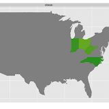
R ggplot - rebuild cdc obesity maps - 1984-2011
redoing the cdc obesity maps with ggplot2

 |
| rebuild cdc obesity maps with ggplot |
Slideshow
- first obese rates
- second overweight rates
- and if the slide show does not work - here is the link to the
pictures
Table of Contents
1 get the data
- I downloaded the data from http://www.cdc.gov/brfss/technical_infodata/surveydata.htm
- for the years 1984 - 1997 I use read.xport() (foreign package) on the sas xpt files
- then the data sets became to large, so I used the ascii files read.fortran() and choose just a few columns
- here is a resulting example data set (2006 - I computed the bmi2 column for checking)
- 2012-09: I added the maps for 2011 since the new data were out
head(x2006)
State month day year age weight height sex htm   wkg  bmi bmigr bmirisk
1     1     5   2 2006  66    263    503   2 160 11955 4669     3       2
2     1     9  19 2006  56    290    603   1 191 13182 3632     3       2
3     1    12  12 2006  40    230    511   1 180 10455 3215     3       2
4     1     4  29 2006  38    320    603   1 191 14545 4008     3       2
5     1     4  29 2006  52    120    504   2 163  5455 2064     1       1
6     1     8   2 2006  32    165    510   2 178  7500 2372     1       1
  heightcm  weightkg     bmi2
1   160.02 119.29417 46.58764
2   190.50 131.54110 36.24695
3   180.34 104.32570 32.07799
4   190.50 145.14880 39.99664
5   162.56  54.43080 20.59763
6   177.80  74.84235 23.67467
2 compute rates and plot the graphs
library(ggplot2)
library(scales)
library(plyr)
library(maps)

## map of the states (part of the map package)
states_map <- map_data("state")
states_map$region <- factor(states_map$region)

## got fips form here and saved it as txt; http://www.epa.gov/enviro/html/codes/state.html
fips <- read.table("states.txt",sep="\t",header=T)
fips$State.Name <- tolower(as.character(fips$State.Name))

## build the graphs

filenames <- paste("bmi",1984:2010,".rdata",sep="")
for(file in filenames){
  load(file)
  year <- substr(file,4,7)
  x <- get(paste("x",year,sep=""))

  ## for adding the year to the plot
  testdf <- data.frame(x2=-70,y2=49,year=year)
  ## for the first 4 years was no bmi in the data set
  ## I named my computed one "bmi" so I need another "bmi2" for the loop, not very sophisticated,
  ## but it works

  if(!("bmi2" %in% names(x))){
    print(file)
    x$bmi2 <- x$bmi
  }

## bmi groups
  x$bmi2gr <- cut(x$bmi2,breaks=c(0,25,30,300),include.lowest=T,labels=c("1","2","3"))

## count
  x <- ddply(x,.(State),transform,perstate=sum(!is.na(bmi2)))
  x <- ddply(x,.(State,bmi2gr),transform,perstate.gr=sum(!is.na(bmi2)))

  dats <- unique(x[,c("State","bmi2gr","perstate","perstate.gr")])
  dats <- dats[!is.na(dats$bmi2gr),]

## percents
  dats$perc <- dats$perstate.gr/dats$perstate
  dats$ow <- as.numeric(dats$bmi2gr) > 1

## I just want the obese and overweight
## >= 25
  dats2 <- dats[dats$ow==T,]
  dats2 <- ddply(dats2,.(State),summarize,perc=sum(perc))
  dats2$gr <- "ow"

## >= 30
  dats3 <- dats[dats$bmi2gr=="3",c("State","perc")]
  dats3$gr <- "obese"

  dats <- rbind(dats2,dats3)

## identify the states in the data set using the region names in the map (fips coded)
  dats <- merge(dats,fips[,2:3],by.x="State",by.y="FIPS.Code",all=T)
  dats$gr[is.na(dats$gr)] <- "obese"
  dats$State.Name <- factor(dats$State.Name)

## graph
  ggplot(dats[dats$gr=="obese",],aes(map_id = State.Name)) +
  geom_map(aes(fill=perc),colour="black",map = states_map) +
  expand_limits(x = states_map$long, y = states_map$lat) +
  scale_fill_gradientn(limits=c(0.1,0.7),colours=cols,guide = guide_colorbar(),na.value="grey50")  +
  geom_text(data=testdf,aes(x=x2,y=y2,label=year),inherit.aes=F)

## save image
  ggsave(file=paste("obese",substr(file,4,7),".png",sep=""))
}
output
[1] "bmi1984.rdata"
Saving 12.7 x 7.01 in image
[1] "bmi1985.rdata"
Saving 12.7 x 7.01 in image
[1] "bmi1986.rdata"
Saving 12.7 x 7.01 in image
[1] "bmi1987.rdata"
Saving 12.7 x 7.01 in image
Saving 12.7 x 7.01 in image
Saving 12.7 x 7.01 in image
Saving 12.7 x 7.01 in image
Saving 12.7 x 7.01 in image
Saving 12.7 x 7.01 in image
Saving 12.7 x 7.01 in image
Saving 12.7 x 7.01 in image
Saving 12.7 x 7.01 in image
Saving 12.7 x 7.01 in image
Saving 12.7 x 7.01 in image
Saving 12.7 x 7.01 in image
Saving 12.7 x 7.01 in image
Saving 12.7 x 7.01 in image
Saving 12.7 x 7.01 in image
Saving 12.7 x 7.01 in image
Saving 12.7 x 7.01 in image
Saving 12.7 x 7.01 in image
Saving 12.7 x 7.01 in image
Saving 12.7 x 7.01 in image
Saving 12.7 x 7.01 in image
Saving 12.7 x 7.01 in image
Saving 12.7 x 7.01 in image
Saving 12.7 x 7.01 in image
Subscribe to:
Posts
(
Atom
)